"The Greatest Equation of All Time"

Sorry to have been so long away from the blog! The purpose of this post is to give some intuition for Euler's identity, "the most beautiful theorem in mathematics", to those who haven't seen it before or to those for whom it is meaningless because they lack the mathematical background.

It was never introduced to me in any class, and unless you majored in math or physics the same is probably true for you. I wanted not only to call your attention to this equation, but also to derive it, the derivation of which is equally marvellous. Walking through the derivation with a pencil was perhaps my first real taste of what I imagine mathematicians live and breathe for; my present aim is to give you a taste!

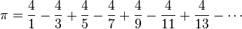
Here it is:

It's pretty astounding when you look at it for the first time... it seems a ridiculous assertion! (However, Gauss is supposed to have said that if this was not immediately apparent to you on being told it, you would never be a first-class mathematician.) He also had a really cool signature, so he is probably right.

Really though? Are we talking about e (2.71828...), like from continuously compounded interest? You mean π (3.14159...), like a circle's circumference-to-radius ratio? And the imaginary number i, the square root of -1, that we talked about for like a week in high school and then never actually used for anything? Yep, those are the ones, e, π, and i. Dust off your old TI-8x, punch this badboy in, and see what output you get. The batteries are probably dead so I'll spare you the trouble:

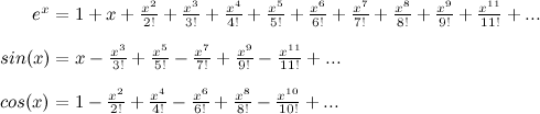
Though I am mainly interested in showing you a way to get to this shocking identity, I will need thereby to talk a bit about Taylor series approximations. If you don't know much about this technique, think of using a sum of polynomials to approximate the shape of function at a given point. If you don't know much about polynomials and functions, think of adding together easy-to-compute things (x, x², x³, ...) to approximate hard-to-compute things (e^x, sin(x), ln(x), ...). This is actually how your calculator computes with things like e, π, et al. 

But this isn't a post about Taylor series approximations, so I'll cut down on the details. If you already understand how to use Taylor series approximations, you could skip to the derivation. If you aren't, it is super useful and cool, so check it out! First things first: if you want to approximate the shape of a function f(x) using an easier-to-work-with polynomial like a power series (i.e., a + bx + cx² + dx³ ... where a, b, c, d,... are constants), you can do it like this:

where f⁽ⁿ⁾(0) represents the nth derivative of function f(x), evaluated at x=0 (this gives us the shape around x=0) Technically, this is a Maclaurin series. Really cool! Because if we can keep taking derivatives, we can get an almost perfect approximation of f(x) using polynomials instead. Don't worry, I'm not going to ask you to do any calculus (though you might want a helpful refresher on derivatives*). I'll just show you the results.

To follow the derivation, you just need the following 3 results: the derivative of sin(x) is cos(x), the derivative of cos(x) is -sin(x), and the derivative of e^x is itself, just e^x.

Let's do sin(x) first, because I've got some pretty pictures of it!

We want to approximate this function using a Taylor series polynomial. Let us do so by taking the first term of that big equation above:

So using only 1 term, our approximation is the line y=x

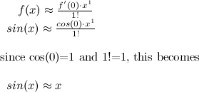
Not a very satisfying approximation, is it? What about 2 terms?

If we plot x - x³/3!, we get

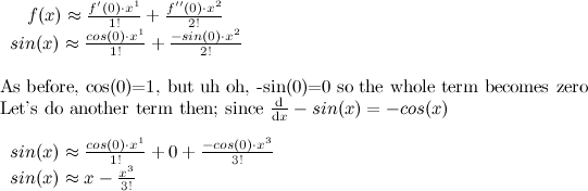
Hey wow, that's a lot better! The polynomial x - x³/3! seems to pretty exactly mimic sin(x), at least around x=0. Let's add another term.

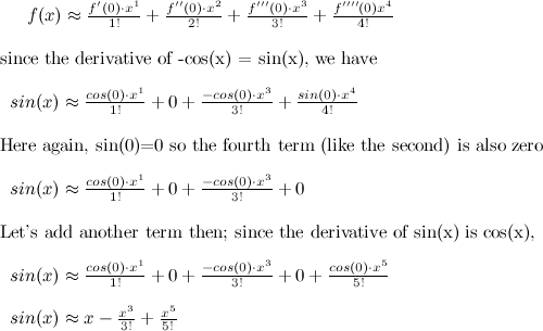
Now our approximation is y = x - x³/3! + x⁵/5! which looks like this:

Even better! You can see that by adding more terms of the Taylor polynomial, we get a closer approximation of the original function. Here's a couple more terms just to illustrate:

Now the polynomial approximation is virtually indistinguishable from sin(x), at least at from x=-pi to x=pi. Here's a more "moving" display of this (credit). Notice how adding more and more terms gets us an ever-better approximation of sin(x).

Here's an even easier example! (We are going to need this result too.)

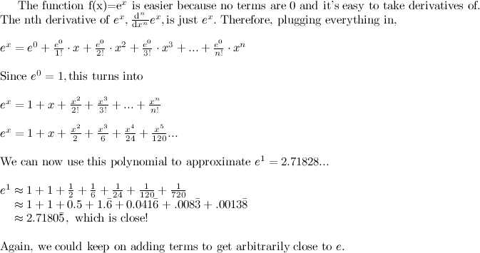
So we have Taylor series approximations for sin(x) and for e^x. Now all we need is one for cos(x). It is just like sin(x) except all of the opposite terms cancel out! I'll leave this as an exercise to the reader (always wanted to say that!) and just give you the result:

Take a minute to look at these. Strange, isn't it? If it weren't for those negative signs, it looks like simply adding sin(x) and cos(x) would give us e^x... Hmmm.

We are now in a position to make some magic happen, but one more thing remains to be done. Now's the time to recall your imaginary number i, which is equal to √−1. Since i = √−1, we know i² = -1. For higher powers of i, we have the following pattern:

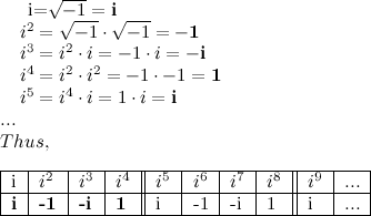
The pattern i, -1, -i, 1, repeats as you take ever higher powers of i. Notice that the signs are switching too! You should be excited about this. Now we're ready for the main event!



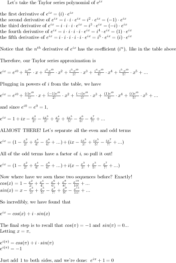
YEAH! WOOHOO! At least, that's how I felt when I first saw it.

And it's not just superficially beautiful either. Before we plugged in pi, we saw that e^ix=cos(x) + i*sin(x). This formula has many important applications, including being crucial to Fourier analysis. For an excellent introduction, check this out.

Well, I hope that if the derivation didn't leave you reeling in perfect wonderment, you were at least given something to think about! Thanks for reading!
________________________________________________________________
*Quick derivatives refresher
It may be helpful to think of the derivative of a function f(x)---symbolized as d/dx f(x) or f'(x)---as a machine that gives of the slopes of tangent lines anywhere along the original function: if you plug x=3 into f'(x), what you get out is the slope of a line tangent to the original function f(x) at x=3. Since slope is just rise-over-run, the rate at which a function is increasing or decreasing, the derivative gives as the rate at which the original function is increasing or decreasing at a single point. If f(x) is the parabola x2, then its derivative f'(x) is 2x. At x=0, the very bottom of the parabola, we get f'(0)=2(0)=0, which tells us the line tangent to x2 at the point x=0 has zero slope (it's just a horizontal line). At x=1, the parabola has started to increase; the rate it is increasing at that point (the slope of the line tangent to that point) is f'(1)=2(1)=2; so now we have a line that goes up 2 for every 1 it goes over. At f'(2)=2(2)=4, a line that goes up 4 for every 1 it goes over. This agrees with our intuition when we look at a parabola; it is accelerating upward at an ever increasing rate.

"Important Peculiarities" of Memory

In my high school psychology class I was told that human memory capacity was unlimited ...and it has bothered me ever since. How, I mean? Aside from the physical limitations on information storage, how could a system that remembers everything forever be evolutionarily advantageous?

This is a question I hope to explore in a deeper way sometime soon; for now, I want to talk to you about a few "peculiarities of human memory" that begin to shed some light on the situation (Bjork & Bjork, 1992). Know that I am drawing heavily from this source and their Theory of Disuse for the present discussion. This is really the coolest part, but I've left it until the end. First, let's talk about three "peculiarities"...

1. STORAGE AND RETRIEVAL ARE TWO DIFFERENT THINGS:
Analogies of human memory -- to a bucket being filled, to computer memory, to magnetic tape -- are often grossly misleading. No literal copy is recorded when you store a piece of information in memory. Learning isn't opening a drawer and putting something in; remembering isn't opening a drawer and taking something out. Indeed, your brain is not a drawer.

New things are placed into memory via their semantic connections to things already in long-term memory. The more knowledge you have of a given area, the more ways you have to store additional information about it. This is a strange biological instantiation of the Matthew effect, where "the rich get richer". To me, one of the most incredible things about being a living, thinking human is this virtually unlimited capacity for storing new information. And when I say "incredible," I mean it both in the sense of "wow, golly!" as well as in the more literal sense of "not credible."

"But wait," I hear you ask, "if my memory is so bally infinite, why can't I remember my passwords half the time? And I'm always forgetting peoples' names, and I can't remember a single word of that book I read last week, and..." As it turns out, getting information into memory is easy, but getting it out is quite another matter.

Quick, what was your childhood address? Your first cellphone number? Your seventh grade math teacher's name? Your high school ID card number? How about your old AIM password? Even the most repetitively drilled, frequently accessed pieces of information eventually become inaccessible through years of disuse. Weirdly though, this information is still stored in memory: you could probably correctly identify each of the above from a list of distracters, for example, and you probably wouldn't have any trouble remembering if you were back in the context of your home town. Perhaps if I had asked you on a different day, when you were in a different mood or frame of mind, you would've been able to retrieve the information. Often information that is effortlessly recallable on one occasion can be impossible to recall on another. Maybe you weren't able to muster the answers at first, but now after expending a bit of time and effort you have remembered. Should the old information become pertinent again, it will certainly be relearnable at an accelerated rate.

What we can and cannot retrieve from memory at any given time appears to be a function of the cues that are available to us at that time. These "cues" may be general situational factors (environmental, social, emotional, physical) as well as those having a direct relationship to the to-be-retrieved item. Cues that were originally associated in storage with the target item need to be reinstated (physically, mentally, or both) at the time of retrieval.

The main takeaway here is that our capacity for storage is far greater than our capacity for retrieval, and it appears that fundamentally different processes are responsible for each. Storage strength represents how well an item is learned, whereas retrieval strength indexes the current ease of access to the item in memory. These two strengths are independent: Items with high retrieval strength can have low storage strength (e.g., your room number during a 5-day stay at a hotel).

2. RETRIEVAL MODIFIES THE MEMORY!
The mechanical analogies have other flaws; reading from computer memory does not alter the contents, whereas the act of retrieving information in human memory modifies the system. When you remember something, that piece of information becomes easier to remember in the future (and other information becomes less retrievable). This is why taking tests is better for long-term retention than studying is. More odd is the idea that recalling Thing A can make it more difficult to recall Thing B in the future, an effect sometimes known as "retrieval competition." This topic is very, very interesting but that's all I'm going to say about it here. For more on the testing effect, check out this paper.


3. LONG-HELD MEMORIES ARE HARD TO REPLACE
Through disuse, then, things become hard to retrieve. But oddly, the earlier the memory was constructed (i.e., the older it is), the more easy it is to access relative to related memories constructed later. Say you decide to change your email password; after doing so, the new password will be the most readily accessible of the two. If you use it to log in tomorrow, you will have little trouble recalling it. However, if you do not have occasion to use either password for a while (new or old), the old password becomes far easier to remember relative to the new password.

Consider athletes: a long layoff often leads to the recovery of old habits. This can help an athlete recover from a recent funk, or it can be a major setback for a rookie who has been rapidly improving. In occupational settings too, and even the armed services, people can appear to be well-trained but then turn around and take inappropriate actions at a later time (i.e., fall back on old habits), particularly in stressful situations. It may even result in the unreasonable surprise we often feel when we see that a child has grown, or a friend has aged, or a town has changed; perhaps we are overestimating these changes because our memory of the child, friend, or town is biased toward a past version of them stored more securely in memory.

This stuff has firm support from laboratory studies too, but I don't want to bore with great detail. Suffice it to say that, if experimental subjects are given a long list of items to memorize and then afterwards asked to recall all of the times that they can remember, there will be a strong recency effect: the items later in the list will be more easily recalled. If, later on (say a day or a week later), subjects are asked to recall all of the items they can remember, there will be a strong primacy effect: the items appearing first will be better recalled than the items appearing later. That this, with the passage of time there is a change from recency to primacy. This finding holds across different delays, tasks, materials, and even species (Wright 1989)!


The Theory of Disuse:
In brief, Bjork and Bjork's (1992) theory states that items of information, no matter how retrievable or well-stored they are in memory, will eventually become nonrecallable if they are not used enough. This is not to say that the memory has decayed or been deleted... it is just inaccessible. Storage and retrieval are two very different things; storage strength reflects the how well-learned the item is, while retrieval strength represents how easy it is to access the item. Unlike storage capacity, retrieval capacity is limited; that is, there are only so many items that are retrievable at any given time in response to a cue or set of cues. As new items are learned, or as the retrieval strength of certain items in memory are increased, other items become less recallable. These competitive effects are generally determined by category relationships defined semantically or episodically; that is, a given retrieval cue (or cues) will define a set of associated items in memory, and the dynamics of competition for retrieval capacity take place across the set.

The theory makes many predictions that account for those peculiarities stated above. Retrieval capacity is limited, not storage capacity, and the loss of retrieval access is not a consequence of the passage of time per se, but of the learning and practice of other items. Retrieving an item from memory makes it easier to retrieve that item in the future but makes it more difficult to retrieve other associated items. The theory also explains why overlearning (additional learning practice after perfect performance is achieved) slows the rate of subsequent forgetting: perfect performance is a function of retrieval strength (which cannot go beyond 100%), whereas additional learning practice continues to increase storage strength. Finally, the spacing effect--the fact that spreading out your study sessions is far more effective for long-term retention than is cramming--can be accounted for by the theory as well. Spacing out repetitions increases storage strength to a greater extent than does cramming, which in turn slows the rate of loss of retrieval strength, thereby enhancing long-term performance. Importantly, cramming can still produce a higher level of initial recall than that produced by spacing, but like the switch from recency to primacy, the switch happens rather quickly.

Again, to spin an evolutionary just-so story, all of this seems pretty adaptive. It is sensible that the items in memory we have been using lately are the ones that are most readily accessible; the items that have been retrieved in the recent past are those most relevant to our current situation, interests, problems, goals... and in general, those items will be relevant to the near future as well. To keep the system current, it makes good sense that we lose access to information that we have quit using: for example, when telling someone our address, it would not be useful to recall every home address we have had in the past.

I look at all of this and I see a selection process at work. The set of items in memory is like so many species in an ecosystem; introduce a new species, and it will die unless it finds a niche (new information must be learned well enough to make it into long-term memory in the first place). Some species don't have much to do with one another, whereas others are mutually dependent and others in direct competition (increasing the retrieval strength of one item reduces the retrieval strength of other, related items). Species with low fitness diminish relative to those with high fitness because they cannot stay  competitive (the items that are used the most proliferate at the expense of items that don't, the item's fitness being determined by the history and recency of its use). Longer, more established species are better adapted to their environment and thus tend to outcompete newcomers (older, more well-connected items memory are easier to recall than newly learned items lacking a deep connection to other items in memory). Species die out, but rarely go completely extinct; instead, they can emigrate elsewhere. They are still extant, but no longer part of the active ecosystem. When conditions improve and it becomes adaptive to return to the ecosystem again, the species is easily reinstated. My metaphor falls apart in places, but I find the selection scheme a good jumping of point for most discussions of this nature.

2 x 2 Statistics

Modern data analysis has gotten very complicated! Let's forget all that for a moment. I wanted to take this opportunity to examine several useful statistical techniques and measures of association that involve nothing more than a 2 x 2 contingency table. A 2 x 2 contingency table (also called a cross tabulation or cross tab) is a simple grid that displays the frequency distribution given two variables--one variable for the columnsand one variable for the rows. Suppose, for instance, that one variable is sex (male or female) and one variable is handedness (right- or left-handed). Lets say we took a random sample of 100 people and determined both their sex and their handedness. We could then take this data and create a contingency table. There are 2 possibilities for sex and 2 possibilities for handedness, resulting in 4 unique combinations: right-handed males, right-handed females, left-handed males, and left-handed females:

	Right-handed	Left handed	total:
Male	43	9	52
Female	44	4	48
total:	87	13	100

Here, if the proportions of individuals in different columns vary significantly between rows (or if the proportions in different rows vary between columns), we say there is a "contingency" between the two variables, and thus they are not independent of each other. This is multivariate statistics in its most basic, two-variable form, but many useful analyses arise from it. Chances are good that you've heard of most of them, and you may have even had occasion to use a few of them before! They are often spotted on the fringes of SPSS output but rarely ever talked about. But many can be quite useful! I'm going to talk about Chi-squared tests, Fisher-exact tests, odds ratios, and several approaches to the humble correlation coefficient (Phi, Rho, biserial, point biserial). Take a look!

Chi-Squared Test

	Q1 Right	Q1 Wrong	total:
Q2 Wrong	a	b	a+b
Q2 Right	c	d	c+d
total:	a+c	b+d	a+b+c+d=N

The above table provides a framework for the examples here to come. Let's say we give a test consisting of just 2 questions (Q1 and Q2) to a total of N students: in the table above,  a is the number who got Q1 right and Q2 wrong, b is the number who got both Q1 and Q2 wrong, c is the number who got both Q1 and Q2 right, and d is the number who got Q1 wrong and Q2 right. Thus, a+b+c+d = N. Also note that a+c is the total number of students who got Q1 right, b+d is the total number who got Q1 wrong, a+b is the total getting Q2 wrong, and c+d is the total getting Q2 right. These numbers are found along the margin of the contingency table.

Now, let's say we were interested to know whether students who got Q1 correct were more likely to get Q2 correct; that is, we want to know if scores on Q1 are correlated with scores on Q2. Let's say we give the test to N=100 students, and here are their scores:

	Q1 Right	Q1 Wrong	total:
Q2 Wrong	14	35	49
Q2 Right	41	10	51
total:	55	45	100

 To assess whether or not there is a relationship between scores on Q1 and Q2, we are essentially asking whether, within each column, the rows differ significantly, or vice versa: within each row, do the columns differ? Well, what would it look like if there were no differences?

	Q1 Right	Q1 Wrong	total:
Q2 Wrong	?	...	49
Q2 Right	...	...	51
total:	55	45	100

Start at the top rightmost cell (Q2 wrong, Q1 right). Assuming that we know only the totals, we would expect that since 49/100 (49%) of students got Q2 wrong, and since 55/100 (55%) of students got Q1 right, then 49% of 55% of the 100 students got Q2 wrong and Q1 right. Thus .49*.55*100 = 27 students. Using the totals, we can subtract 27 to calculate all of the other frequency values:

	Q1 Right	Q1 Wrong	total:
Q2 Wrong	27	22	49
Q2 Right	28	23	51
total:	55	45	100

 These are the frequencies we would expect to get if Q1 and Q2 were independent of each other (that is, uncorrelated). But this is not what we saw!

To see if these expected frequencies are significantly different from the numbers we observed, we compute a chi-squared test statistic like so:

Thus, for each cell, we subtract the expected frequency from the observed frequency, square that quantity, and divide by the expected frequency. Then we add them all up. This gives us a measure of how much our sample deviates from the expectation.

Our test statistic is 27.3; this seems big, but we need to look at a chi-squared distribution with (#rows-1)*(#cols-1) degrees of freedom. Here, that's just 1.
Instead of going to a table of critical values, I'll use R to make a pretty graph:

 > qchisq(.95,1)  
 [1] 3.841459  
 > cord.x<-c(0, seq(0.001,3.84,.01),3.84)  
 > cord.y<-c(0,dchisq(seq(0.001,3.84,.01),1),0)  
 > curve(dchisq(x,1),xlim=c(0,10),main='Chi-Squared, df=1, a=.05')  
 > polygon(cord.x,cord.y,col="skyblue")  

If the data were independent, there is a less than 5% chance of observing a test statistic larger than 3.84; our test statistic was much larger, 27.3! Thus, it is extremely unlikely that we would observe a value that large if our data were uncorrelated. So, we reject that possibility.

Another, perhaps quicker way of computing the chi-squared test statistic is worth mentioning here.

Check out the squared quantity on top: look familiar? You've got a determinant here! If that quantity (ad-bc) were zero, you would know that responses to the two questions were perfectly independent. It would also be the case that the 2x2 table is "rank one", meaning that all rows are scalar multiples of the first nonzero row. To illustrate this briefly,

	Q1 Right	Q1 Wrong	total:
Q2 Wrong	4	3	7
Q2 Right	8	6	14
total:	12	9	21

Multiply the top row by 2 to get the bottom row, right? Also ac-bd = 24-24=0. So here there is no association between scores on Q1 and on Q2.

But wait, back to our original example.

Measuring the extent of the relationship with correlations:

 Phi coefficient

Once you have your chi-squared test statistic, and you know that there is a relationship between your two categorical variables, you can easily use this number to calculate phi, which results in the same value as a correlation coefficient. If we take our chi-squared test statistic (27.3 above), divide it by the total number of people, and take the square root of that quantity, we get  the phi coefficient:

Doing this here yields sqrt(27.3/100)=0.522, which is a moderate correlation. Note that this is exactly the same value as would Pearson's r. Here's a helpful table to help you pick the measure of association that's right for you!

	Continuous	Ordinal	Categorical
Continuous	Pearson's r	-	-
Ordinal	Biserial r	Spearman's ρ; polychoric	-
Categorical	Point-biserial r	Rank Biserial	Phi (φ)/Matthews

Odds Ratios

	Q1 Right	Q1 Wrong	total:
Q2 Wrong	14	35	49
Q2 Right	41	10	51
total:	55	45	100

An odds ratio is another way of quantifying the size of the effect detected by chi-square significance tests of dichotomous variables. Think of the "odds" of an event as the probability of the event happening divided by the probability of it not happening. If you got Q1 right (first column), the odds of a correct answer on Q2 are (41 right)/(14 wrong), or 2.93, meaning that almost 3 times as many people got it right as got it wrong, so getting it correct is 2.93 times as likely (the odds are 2.93 to 1). We can calculate other three 'odds' in the same manner; of the people who got Q1 wrong (second column): 35 got Q2 right and 10 got Q2 wrong, so the odds of a right answer to Q2 given you got Q1 wrong are (10 right)/(35 wrong)=.29; thus, if you get Q1 wrong, you are more than three times as likely to get Q2 wrong than you are to get Q2 right.

Now, the odds ratio is just what it sounds like: the odds of an event happening in one group divided by the odds of it happening in another group. The ratio of two odds tells us how much more likely an event is to happen in one group versus another. Using the calculations above, we can ask, "how much more likely are the students who got Q1 right than those who got Q1 wrong to get Q2 right ?" To do this, divide the first odds of a correct Q2 of the first group (those who got Q1 right) by the odds of a correct Q2 of the second group (those who got Q1 wrong). Doing so yields (2.93/0.29)=10.1, which means that those who got Q1 right are 10 times more likely to get Q2 right than are those who got Q1 wrong.

If an odds ratio is greater than 1, then "A" is associated with "B" in the sense that having "A" raises the odds of having "B" (relative to not having "A"). In the present example, "Q1 Right" raises the odds of "Q2 Right" (relative to "Q1 Wrong").

Fisher's exact test

OK, quick aside. Imagine you have an urn containing 10 balls; 3 of them are black and 7 of them are red. If you choose 5 balls at random, what is the probability that all 5 are red?  If you know a little about combinatorics, you know that there are "10 choose 5", or 252 ways to choose 5 balls from 10:

 

This tells us that there are 252 unique 5-ball combinations; now how many of those have 5 red balls and 0 red balls? Well, how many such combinations are there? How many ways are there to choose 5 red balls from 7 red balls? Say "7 choose 5". Now, how many ways are there to choose 0 black balls from 3 black balls? "3 choose 0." The product of these two combinations (7 C 5) and (3 C 0) give us the number of possible 5-ball combinations in which all 5 are red (and zero are black). 

Now then, these what proportion of the total number of possible 5-ball draws (total=252) will have 5 red and 3 black (total=21)? Well,

 

Where N is the total number of balls in the urn, R is the total number of red balls in the urn, n is the total number we select, N-R is the number of black balls in the urn, r is the number of red balls in our selection, and n-r is the number of black balls in our selection. Experiments of this kind follow a hypergeometric distribution, we can this method to analyze our 2 x 2 contingency table.
Now, instead of balls and urns, we have right and wrong. Instead of asking, "what is the probability of getting 5 red balls and 0 black balls when I draw 5 balls at random from a population that contains 7 red balls and 3 black balls" we ask "what is the probability that 14 people got Q1 right/ Q2 wrong and 35 people got Q1 wrong/ Q2 right if we draw 49 balls at random from a population where 55 got Q1 right and 45 got Q1 wrong." That is, we want the probability of observing the given set of frequencies 14, 35, 41, 10 in a 2x2 contingency table given fixed row and column marginal totals.

	Q1 Right	Q1 Wrong	total:
Q2 Wrong	14	35	49
Q2 Right	41	10	51
total:	55	45	100

 

This probability is vanishingly small, but what we are really interested in is this: given our marginal frequencies, what is the chance of observing a difference at least this extreme? More extreme configurations can be generated by locating the smallest (or largest) frequency in the table, subtracting 1 (or adding 1), and then computing the remaining items given the observed marginal frequencies. When you find the collective probability of observing a combination of frequencies at least as extreme as this one, you get something smaller than 1/10,000,000. Thus, we can conclude that answering question 1 right is associated with answering question 2 right.

Fisher's exact test is interesting because it depends on no parametric assumptions and works for any sample size.

I may add more to this post in the future, but that's enough for now!

The Math of Secrecy: RSA Cryptography (and Shapes You Can Draw?)

When Gauss was 19, he discovered that of the infinite number of polygons that have a prime number of sides, a mere five of them can be constructed with a ruler and compass (i.e., using only straight lines and circles). These prime-sided polygons can have 3, 5, 17, 257, or 65537 sides, but only these five are possible (probably).

Indeed, the only shapes you can draw with an odd number of equal-length sides are the multiples of these 5 Fermat primes: 3, 5, 15, 17, 51, 85,..., 4294967295
(amazingly, all constructable polygons must have a number of sides that is a multiple of a Fermat prime and a power of 2!). There are good reasons why this is true, but they are confusing and would belabor this post.

Apparently, Gauss was so happy with his finding that he requested a regular heptadecagon on his tombstone; the stonemason declined, stating that it would essentially look like a circle. After watching the requisite process below, one begins to sympathize with the stonemason (diligent wikipedian Aldoaldoz made both of these; in case you want to build your own 17-gon, you can break out the compass and follow along at home). It's hypnotically beautiful, but the .gif alone is 462 frames and takes a full 1:26 to watch...

These strange numbers are known as Fermat primes, and take the form 2²ⁿ+1. Though there are infinitely many numbers of this form, only the first 5 (above) are prime. As I was reading about these yesterday, I found that they have an important application in the most common form of public-key cryptosystems, whereby messages are encoded so as to conceal their meaning.

This method of encryption is used to secure electronic communication over the internet; even if a third party somehow manages to nab your encrypted message, it will be almost impossible for them to crack it. If you've used SSH, SSL/HTTPS, PGP, or had to verify a digital signature, you've used RSA encryption or one of its descendants.

On personal websites, you may have run into these before:

-----BEGIN PGP PUBLIC KEY BLOCK-----
Version: GnuPG v1.4.11 (GNU/Linux)

mQENBFPCyXEBCACuHid62W3FI3DegXw3G6Xyjdj3SBl3+f/fBNIN4Yrx0auPjuZG
TqtA6opOH7jzAEBdBBysiQ+1frQlfiWlmdzJ/GQR7KGhuZNx33pyCwXV85bcKtno
A4CQK8r2sfrRF796voNWxW/MaStT7IWQfHrMYsgcl+7cZogBu/nl3nnHuZz+oMMG
ZZl+uziKF1+M4naOr6gH3UMTECk2Xib2lk58RFN4pmqPzbWG5gUU5ugN13c6hO7S
eKN/cbGSHRHPQci0aZo743rIoWgQZ+S88j3BweGFbD78tw5UYJUW+rnyYISzDbVi
R+i8luzVtVhkHZnetcQoz6IBsDyfnK0dKMLhABEBAAG0K05hdGhhbmllbCBSYWxl
eSA8bmF0aGFuaWVsLnJhbGV5QGdtYWlsLmNvbT6JATgEEwECACIFAlPCyXECGwMG
CwkIBwMCBhUIAgkKCwQWAgMBAh4BAheAAAoJEH4levi+sCboeHoH/3IyNGGwxVWy
VVnjKj2vpbgysU4W4xieL9sWvMBFnKDhpHZsazBEhXnmhEbDouixZaFeMmul8C7J
2/5Ljync/fkPCKtyF+Ibovs3ALuHnY4Iu8vukxMbr7cmB1lOkVGxHIKcjGX4H9F7
6qnGYmJWpz+pgYIbq5xO07aCcwE9/EUQwh0MdDml0euRiDWio1HOM7XTVJJ7AmyX
MKroqF+Ik/93mSl4vGlKKqDhPr3hcxqFsE8LhHgMxeI2NGomhka064mwWqRpFf0f
ce33cWaFSgl+rRAqkQkZUdiMnbIj9P89OH/PqOQgaB/nXIVXmjMb6HluhJA/2ZnM
h+Y8e0pF2j+5AQ0EU8LJcQEIAK38D6Bnho1cennrFOVcCj1nmlG4UW9mWr2ox+WJ
QBEqw8IUsWg/0LEe5K3MPoOE3lO3VTHnKqLMJSbA9byjSwYxIE3Y1QoY1Uq43Da1
sYkeETVkMgnAGmIwSQgsdfdAGhXv5uF/Ck3O+QMdUW5qZ4s+WXUCMWcj4ZgomUxC
i0bQgE/w/TDc0JAisma2oOuOTVjpfyX5VCk6XtwmDxE+STHZTCIKvSnyodx3Hlke
1gr+f/ejpbAnYiyjjWpiQGS47YCjAzGAsn0CRJ4dQYsjv6RVL/O/EYEJDUs49cLW
ccYhj0BQZyeMqWxZqP8ZUIGsoPfzh/ahLNXnxlqVTD53eA8AEQEAAYkBHwQYAQIA
CQUCU8LJcQIbDAAKCRB+JXr4vrAm6OFPB/9P4GkEV+XpejL4TO17Sh7vj3nZvKxd
AoPKKG1qbJNuYqasz0d5C0hfZN4aLaKdiWide9sIMfjRrG1gbN8o34uR3i3887Eg
zrhZWS/E01jGqR4ey/iACyfXvDfEFEwthfChyS9qQVYw7fWWSBtpZqJ5iul7Jf7b
tHPeqizK2FqOSnJy9ovaHHcZL4Wt26Y+IDWq0WQKB89guhN6LhlaQQXrAhlbwW2N
DcvTrHm3g4sVxeuAujGJzJGRmf5hkV+YxG2OrpLQjx+n4XsZSFO3tdfNwTwDn1Xj
9AFqGhRzm9j1Cq3iqcTbJtQwwJknkNm7CLFeHuy4zurzP3gmwnRvZ2UM
=X1Q+
-----END PGP PUBLIC KEY BLOCK-----

To the untrained eye someone's cat has been traipsing about on their keyboard, but in reality this string represents two (big, random) numbers that allows you to communicate with it's provider in a completely secure fashion. It is a "public key" and is used to encrypt messages sent to its owner; it has a mathematically precise twin, a "private key" which only the owner has access to. This private key is required to decode the message originally encoded by the public key.

For an extremely helpful analogy, consider a padlock. A public key can be thought of as an open padlock and a private key is the key that can unlock it once it is closed. In public key cryptosystems, you give your close friends copies of your personal padlock, open and unlocked (this is your public key). They can now send you messages securely by locking them in a box using your padlock (i.e., encrypting it with your public key) and sending it to you, because only you have the key (the private key) which can open it. Note that your friends don't need a key to close the padlock: they simply put their message in the box and shut the padlock.

How does this work mathematically? Here's a technically correct but very basic run-through of RSA for didactic purposes:

Let's say you want to communicate privately with another party. They're going to send you a secret message (message: "PRIVATE") over the internet, and they want to be sure that no one else can read it. In order to do so, they can encrypt this message using your public key and send it to you; you can then use your private key to decrypt and read it.

Let's assume you haven't yet generated public/private keys, and you want to do so by hand:

STEP 1
Choose a pair of prime numbers, p and q, at random.
To keep the math reasonable, let's take p=3 and q=17

STEP 2
Multiply p and q together to get their product n.
Here n = 3 x 17 = 51 (This is the step that is hard to reverse in practice!)

STEP 3
Multiply (q-1) x (p-1) to get the totient of n, φ(n)
φ(n)= (3-1) x (17-1) = (2) x (16) = 32.

STEP 4
For the first key, choose any number e that is smaller than φ(n) and has no common factors with φ(n). Since φ(n) = 32, we can choose any number besides 1, 2, 4, 8, 16, and 32.
Lets pick e =11.

STEP 5
Finally, the matching key d must be computed. This is achieved by "taking the inverse of e modulus φ(n)". All this means is that we need to find the number d to multiply e = 11 by so that when we divide their product by φ(n) =32, we get a remainder of 1. This isn't as hard as it sounds: φ(n)=32, and e=11. Since 11 x 3 = 33, and 33 divided by 32 leaves a remainder of 1, we know that the d, "the inverse of 11 modulus 32" , equals 3.

These keys e=11 and d=3 are mathematically linked through n=51, because
if you take the number you want to encrypt to the power of e and divide by n, you get a remainder. This remainder the encrypted version of your original number. To decode it, just raise it to power of d and divide by n.

As quick example, say the secret message you want to send is the number 4. To encrypt it using our public key (e=11, n=51), do

4¹¹ % 51 = 4194304 % 51 = 13.

The number 13 is our encrypted message, which can only be unlocked if you have the private key (d=3, n=51). The same procedure used to encrypt is used to decrypt, but take 13 to the power of d and find the remainder when dividing by 51.

13³ % 51 = 2197 % 51= 4, our original message

Without factoring n = 51  you can't easily compute φ(n) 32 and thus knowing one key, you can't easily compute the other.



But how do we send the secret message "PRIVATE"? First you should get a numerical representation of this message; commonly, a much longer messages is being sent and it is converted from ASCII to its decimal representation. For now, we can just take the number that corresponds to each letter's position in the alphabet, (A=1, B=2,..., Z=26). Doing so for this message yields "16 18 9 22 1 20 5".

To encrypt our message ("16 18 9 22 1 20 5") using one of the keys (now therefore the public key), we repeat the process used above for the number 4, but now we use it on each of the numbers in our numeric code:

encrypted = original^public_key mod n.

16¹¹ mod 51 = 17,592,186,044,416   % 51 = 16
18¹¹ mod 51 = 64,268,410,079,232   % 51 = 18
9¹¹   mod 51 = 31,381,059,609         % 51 = 15
22¹¹ mod 51 = 584,318,301,411,328 % 51 = 28
1¹¹   mod 51 = 1                               % 51 = 1
20¹¹ mod 51 = 204,800,000,000,000 % 51 = 41
5¹¹   mod 51 = 48,828,125                % 51 = 11

So our encrypted message is (16 18 15 28 1 41 11). This is the message we send to our intended recipient. Even if it is intercepted in transit, it remains unintelligible without the private key.

To decrypt the message, repeat the process except now we are raising the encrypted message to the power of the private key (3), which transforms it back into its original code.

original = encrypted^{(private_key)} mod n.

16³ mod 51 = 4096   % 51 = 16
18³ mod 51 = 5832   % 51 = 18
15³ mod 51 = 3375   % 51 = 9
28³ mod 51 = 21952 % 51 = 22
1³   mod 51 = 1        % 51 = 1
41³ mod 51 = 68921 % 51 = 20
11³ mod 51 = 1331   % 51 = 5

Resulting in the original message, (16 18 15 28 1 41 11 = "P R I V A T E").


The way this works in practice is that you generate your own set of keys, one public and one private. The public key is made known to others with whom you wish to communicate privately (often by posting it somewhere online). Then, if someone wants to send you an encrypted message, they simply encode their message using your public key and send it to you. At this point, the message is garbled and can only be decoded using your private key. Remember that big block of garbled nonsense above? That's my public key, analogous to (11, 51) in the example above except that in decimal form it has over 300 digits!

In the demonstrative example above, our n = 51. Numbers like 51, which are the product of two primes numbers, are called semiprimes. Its not hard to see that 51 = 17 x 3, and these factors are all you need to crack our code! So how is this secure? The strength of the security offered by RSA and similar cryptographic methods is that finding the original factors of a huge semiprime is computationally difficult. For small semiprimes its no big deal, but when the two prime factors are large (~300 digits, which is more than a "googol"!), randomly chosen, and about the same size, the search becomes impractical for even the most powerful computers. The number of operations required to perform the factorization exhausts all our of present computer power.

The largest RSA number that has even been successfully factored is 768 bits (232 decimal digits), and this took hundreds of computers more than two years to accomplish! Indeed, much smaller RSA numbers, many with large bounties in their day, remain unfactored. Still, this method of encryption is not "uncrackable" and the size of the numbers used will have to stay one step ahead of developments in computing power. There do exist uncrackable codes, however...

Now, why are Fermat primes (2²ⁿ+1) useful in RSA cryptography? Often, the public key exponent is one of these five numbers, typically 65537. Consider their binary representation:

3 = (11)2
5 = (101)2
17 = (10001)2
257 = (100000001)2
65537 = (100000000000000001)2

They are computationally convenient! There are probably other reasons too... let me know if you think of any!

Circling the Square & Squaring the Circle!

In A Mathematician's Lament, Paul Lockhart roundly decries the way our school system sucks the soul out of mathematics; what was forced down most of our throats was an insipid husk of repetitive calculation, plug-in formulae, and rigid formality, all of which we were called upon biweekly to regurgitate. Most painful for him to see is the way geometry is taught:

"All metaphor aside, geometry class is by far the most mentally and emotionally destructive component of the entire K-12 mathematics curriculum. Other math courses may hide the beautiful bird, or put it in a cage, but in geometry class it is openly and cruelly tortured.
(Apparently I am incapable of putting all metaphor aside.)"

If you haven't read the Lament yet, definitely stop what you're doing and take the next 30 minutes to do so; if you have any interest at all in mathematics or education, it will be one of the best-spent half-hours of your life.

Having deep, abiding interests in both of these things, I was personally moved by the piece and feel a renewed enthusiasm for shapes and numbers, an enthusiasm that was all but aborted by my own early math education. Yours almost certainly was too! Here's what I mean...

          

Consider a line segment 2 units long. Now, make a square where each side is one of these segments. We have "squared" our 1D segment and we got a 2D shape 2 units long by 2 units wide. That's 4 square units total, because 2²=2x2=4. Thus, we say that the area of our square is 4 square units! (Area is just an arbitrary measure of what you get when you compare the shape to squares of a fixed size, in this case 1 square unit.)

We can take these 4 square units and arrange them however we want: if we put them all four in a row, we create a rectangle 4 units wide by 1 unit tall. It has the same area as the square; we can see this by inspection or by noticing that 2x2=1x4. It is true for all rectangles and parallelograms that area = length x width.

Instead of memorizing a formula, how could we find the area of a triangle?
Is there a way we can cut the square to make triangles? Yes, absolutely. Cut a square diagonally and you get two triangles. Are these the same size? Yes! So if two equal parts make 1, we know they have to be half of the original. Thus, the formula you had to memorize in grade school makes some obvious, visually verifiable sense. You were told, "base times height divided by 2" or "one half base times height". Well, now you see that "base times height" gives you the area of a rectangle, and "divided by 2" gives you exactly half of the rectangle's area, corresponding to a triangle.

 

Teaser: how much of the box is taken up by each of the triangles below?

 

Here's a hint:

Answer: It's always half! 

The Diagonal of a Square
Now then, let's take just one of our square units (from earlier). Here's a question: measure from corner to corner diagonally, and what do you get?

       

Well, we can see that it's longer than 1, but shorter than 2. Indeed, 1.5 is a pretty good guess, but it look to be a bit less. 1.4?  A bit more than this. 1.41?

Let's zoom in a bit... Uh oh, we're not quite there. 1.415? Close, but zooming in a bit more we can see we still overshot it. How long is this lousy diagonal line?! It's length doesn't seem to be representable in ordinary integers or fractions...

 
Have we made some mistake? This extremely regular shape has already produced for us a bit of a quandary; we're just trying to measure the length between a square's two corners! It's as if Well, whatever the length is, let make a square out of it too. Two squares might be easier to compare...

Take a minute to look at the two squares. Notice anything? It looks to me like half of our original square fits inside this new square exactly 4 times. 4 halves make 2 wholes, so 2 original squares = 1 new, diagonal square.

Let's see if we can find that diagonal now! We know that two squares whose sides are 1 add up to form a bigger square, whose side we don't know (besides knowing it's close to 1.4). Let's call that side length d, for diagonal. So, we can say 1²+1²=d².

Since 1² is just 1x1, which equals 1, and since 1+1=2, we know that d²=2. This says that our diagonal squared is equal to 2. We are almost there! At this point, you might just take the square root of both sides: the square root of d²= d, and the square root of 2 is, well, √2. So the diagonal of a square with side lengths of 1 is equal to √2.That's not satisfying at all!... what is
this √2 business?


How to Find √2
We know that our diagonal line d, times itself, equals 2, or d²=2, that's just saying that dxd=2, or d=2/d (if we divide both sides by d). We got close earlier just by measuring; we found that the diagonal length was less than 1.5, and probably around 1.4.

Let's let 1.5 be our first guess for d and then see if we can refine our guess to get closer to the answer: so d=1.5... since d=2/d, we should divide 2 by 1.5 to see what we get:

DIVIDE 2 BY OUR GUESS:
2 / 1.5 = 1.3                                                   ....in fractions, 2 / (3/2) = (4/3)

So, we know that 1.3 x 1.5 = 2, but we want 1.3 and 1.5 to be the same number: we want d x d = 2. Our next guess should be a number in between these two numbers, so lets average them! 

GET A NEW GUESS (average the old guess and the quotient):
(1.5  + 1.3) / 2 = 1.416                ....in fractions, ((3/2) + (4/3)) / 2 = (17/12)

Our next guess is 1.416, so we can do this process over again: divide 2 by our guess, and take the average of the quotient and the divisor:

2 / 1.416 = 1.4117647058823529           ....in fractions, 2/ (17/12)= (24/17)

We know the answer is somewhere in between 1.416 and 1.4117647058823529, that is, between (17/12) and (24/17). Average them!
((17/12)+(24/17)) / 2 = 1.414215...                         ....in fractions, (577/408)

If we were to repeat this process forever, we would converge on the square root of 2, which is the length of that diagonal. But until we do an infinite number of these averages, we won't know exactly how long the diagonal of a square is! Unbelievable! Chances are, you've already whipped out your calculator and found that √2  = 1.414213562..., so our averaging method worked well! After just 3 iterations, we're off by only 0.000015%! What does it mean, though that this "irrational" hole to infinity emerges when we try to do something as basic as measure a square? What does it mean?

What about π?

I don't know about you, but no one ever showed me what π (pi) was all about. I mean sure, as far as numbers it is culturally unique in having, for whatever reason, made its way onto t-shirts and bumper stickers like some kind of geek heraldry. we hear over and over again that this 3.14 is some number equal to ~22/7, and know it has to do with circles because we had to memorize that A=π r² and C=2π r. We may even know that it's "the ratio of the circumference to the diameter," which is simply a restatement of the formula ( π=2r/C=d/C). But what is π, what does it look like, and what do these equations really mean? Paul Lockhart discusses the educational disasters that can accompany this topic:

"To help students memorize formulas for the area and circumference of a circle, for example, [teachers will recite] this whole story about “Mr. C,” who drives around “Mrs. A” and tells her how nice his “two pies are” (C = 2πr) and how her “pies are square” (A = πr²) or some such nonsense. But what about the real story? The one about mankind’s struggle with the problem of measuring curves; about Eudoxus and Archimedes and the method of exhaustion; about the transcendence of pi? Which is more interesting... using a formula that someone handed you without explanation (and made you memorize and practice over and over) or hearing the story of one of the most beautiful, fascinating problems, and one of the most brilliant and powerful ideas in human history? We’re killing people’s interest in circles for god’s sake!"

 So let's talk about π, not because we have to memorize it, but because it is weird and fascinating and very much worth thinking about for its own sake!

 Above, we talked about how, when you take a square's diagonal and divide by its side, weird stuff happens (you get √2). Even weirder stuff happens when you measure around a circle (circumference) and divide by the distance across (diameter): you get π. Humans have been refining their calculations of this value since at least 1850 BC. We first noticed that, for any given circle, the distance around a circle is about 3 times the distance across. But as the figure above illustrates, this is not quite right: 3 diameters around almost gets us there, but leaves us coming up short by somewhat more than 14 hundredths. But how much more, exactly?

Around 250 BC, Archimedes came up with a new approach: because we can measure straight lines but not curves, just stick the circle inside a shape made from only straight lines (i.e., a polygon), and increase the number of sides to get closer and closer to a circle. Then measure the straight lines around the outside.



Here's an example of Archimedes' influential technique: put a circle with a diameter of 1 exactly inside a square: Our first guess for the area of a circle is the number of sides of the square times the length of each one (the perimeter of the square), which in this case is 4. To home in our pi, we keep increasing the number of sides and multiplying by the length of each one, as shown above for four more polygons (a hexa-, octa-, dodeca-, and 24-gon). Notice that, even when approximating with a 24-sided shape, our guess comes up pretty short (3.15966). 

Using this method, Archimedes proved that 3.1408 < π < 3.1429. More than 1800 years later, humans were still using this technique: the record in 1630 for calculating digits of π was 39 (this record still stands as the most accurate manual geometric calculation of π).

If you want to calculate these yourself, you need to know the side length of your n-gon. This can be calculated using the tangent function, opposite over adjacent. Since the radius is 1 in our case, we just do tan(π/n) where n is the number of sides*. (This was much more difficult for Archimedes!)

 

*Here's why: dividing π by the number of sides gives us the degree measure of the the top angle in a triangle formed by connecting  the polygon's to the center of the circle. Half of this measure is the angle measure of the right triangle shown above; if we take the tangent of this angle, it gives us the value of opposite/adjacent:  = (s/2)/(1/2) = s. AWESOME! Since  s is our side length, we found that simply taking tan(π/# of sides) gives us the length of one of those sides (in the case where the diameter is 1). In general, the length of the side is found by multiplying tan(π/n) by the diameter.

Infinite Series Calculations of π

This kind of calculation results when a pattern of numbers, being summed or multiplied repeatedly, converges on a mathematical constant (or some fraction thereof).

Though an Indian mathematician named Nilakantha discovered the idea of using an infinite series to calculate π around 1500, they weren't used in the West until the 1600s. Old Nilakantha's  series is actually pretty good:

 

After 4 terms it's at 3.1452...! The first known Occidental series was this one, found by Fracois Viete:

Notice that it is less than ideal because it depends on the square root of two, another difficult number. In the 1670s, the Gregory-Leibniz series was found:

The 20th century gave us computing and iterative algorithms that are calculating ever more digits. Interestingly, it also saw several new infinite series that are faster than these iterative algorithms and less memory-intensive. Ramanujan found this one in 1914:

And in 1987, the Chudnovsky brothers came up with this bad boy, which produces about 14 digits of pi per term!

 

Needless to say, it was used for several record-setting calculations. Including the first to surpass 1 billion digits (1989) the first to surpass a trillion (2009), and 10 trillion (2011).

Area of a Circle

One last thing for now: since we talked about pi, and since we talked about the area of squares (and triangles), we should definitely end with the area of a circle. For this, you probably memorized the formula A=πr², but what does this mean? It means that if we take the radius, make a square out of it, and multiply that square by pi, we have the area. Can we connect this to the way we found the area above, i.e, length-x-width or base-x-height? Absolutely! 

Imagine unpeeling tiny layers from a solid, filled-in circle and laying them side by side until there are no layers left (as in the picture below). The first layer you peel off is a circumference (its length is 2πr) the next layer is a tiny bit shorter, and the next is shorter still, and so on... Eventually, you will have unpeeled your whole circle to form a triangle with a base as long as the radius of the circle and a height as long as the circumference: this is the top triangle in the picture. Well, what's the area of this triangle? (Base x Height)/2, right? So that's radius times circumference divided by 2, or (2πr x r)/2 = πr² = Area!