I've been recently acquainted with a statistical technique of amazing utility and versatility that has its roots in matrix decomposition, a basic---though profound---concept in linear algebra.
For the purposes of this discussion, we're going to consider it a very elegant way of taking a large, confusing dataset with many variables and transforming it so that you can find patterns based on the correlations among the variables, thus allowing you to describe your data with fewer of them.
Though it comes in several of flavors which go by various names, we'll call it Principal Component Analysis (PCA), and later I'm going to show you how you can use it to implement a sort of computer vision/face recognition thing using either Matlab or GNU Octave.
Before this, though, we need to be comfortable with two concepts: (co)variance and eigen-things. If you are already,
SKIP TO PCA or
SKIP TO EIGENFACES (this is a very long post).
______________________________________________________
Variance & Covariance
Look at the two datasets below; both have a mean of 50, but different variances. Even if you are utterly unfamiliar with the concept, try to guess which has more variance (i.e., variability):
{48 43 52 57 50} vs. {10 25 90 75 50}
The numbers on the right are way more spread out from the mean, right? In fact, if you take each number's distance from the mean, square it, and average those values, you get the variance of the data. So, for the one on the left you have
= (48-50)2+(43-50)2+(52-50)2+(57-50)2+(50-50)2
= 4+49+4+49+0
= 106 [sum of squared deviations from the mean]
And on the right side you have
= (10-50)2+(25-50)2+(90-50)2+(75-50)2+(50-50)2
= 1600+625+1600+625+0
= 4450 [sum of squared deviations from the mean]
Now divide both by 5 to get the average squared deviation from the mean
variance for left set = 106/5 = 21.2
variance for right set = 4450/5 = 890
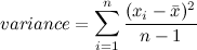
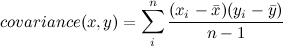
In general, the equation for calculating the variance of a sample of data is
Notice that here, the numerator is exactly what we did above, but the denominator is (
n-1) instead of just
n. In stat-speak, that's because, in our case, we aren't interested in estimating population variance from our sample; if we were, divided by
(n-1) would give a better estimate. In this example, we are effectively treating our sample as a population.
______________________________________________________
Covariance
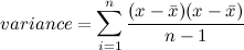
It's helpful to start by thinking of variance this way, expanding the numerator
Variance is only useful when we're dealing with one dimension; often, though, we want to know about relationships between the dimensions. Covariance tells us how much the dimensions vary together:
Seen in this way, variance is just a special case of covariance, where you calculate the covariance of the dimension with itself.
Below are two scatterplots illustrating a linear relationship between two variables; I have included the least-squares line of best fit for each
relationship. Even if you are utterly unfamiliar with the concept, guess
which relationship has more covariance (i.e., how much the variables change together):

The plot on the left shows a much neater, tighter relationship, with changes in one variable corresponding closely to changes in the other (varying
together; heavier people also tend to be taller people); the one on the right, while still having positive covariance (more hours spent on homework tends to result in higher grades), doesn't look quite as tight. A negative covariance would mean that the variables do
not change together; that increases in one are associated with decreases in the other.
The covariance for height and weight is 92.03 and the covariance for homework and grades is 5.13; while we should be pretty convinced by this disparity that height & weight vary together more closely than do homework & grades, in order to confirm this the covariances should be standardized. To do this, we divide each covariance by the standard deviation of each of its variables, resulting in the correlation coefficient, Pearson's
r. For height vs. weight, r = 0.77 and for grades vs. homework, r = 0.33, confirming our observations.
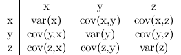
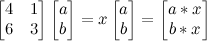
Covariance matrix
If you have three variables (x, y, z), a covariance matrix for your data is just a matrix with each cell being cov(row,column). It would look like this:
You can see that the diagonal consists of the variance of each variable. Also note that a covariance matrix is redundant, because cov(x,y)=cov(y,x). I'll make it look more matrix-y for you:
These will be crucial later, so keep them in mind.
______________________________________________________
Eigenvectors and eigenvalues
In German "eigen" means "self-" or "unique to", giving us some initial clues--we've got a vector that is unique to
something and a value that is unique to
something. That
something is a square matrix (same # of rows & cols). An vector
v is an eigenvector for a square matrix
M if, when multiplied by
M, it yields a vector that is an integer multiple of
v. That is,
Mv=xv, where x is any integer.
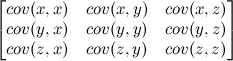
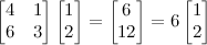
An example should make this clear. Say we have the following square matrix; we want to find the vector [a b] such that x is an integer.
Any such vector [a b] we call an eigenvector of this matrix, and any such integer x an eigenvalue.
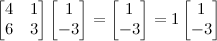
Here, [1 2] is an eigenvector and 6 is an eigenvalue of our matrix. These aren't easy to come by, and solving for them by hand is usually infeasible. An
n x
n matrix will have
n eigenvalues. In this case, 1 is the other, and an example of an eigenvector is [1 -3]. See?
OK, that's probably enough to "get" PCA; just remember covariance matrices and eigenvectors, and you're set.
______________________________________________________
Principal Component Analysis
PCA was independently proposed by Karl Pearson (of r fame) and Harold Hotelling in the early 1900s. It is used to turn a set of possibly correlated variables into a smaller set of uncorrelated variables, the idea being that a high-dimensional dataset is often described by correlated variables and therefore only a few meaningful dimensions account for most of the information. PCA finds the directions with the greatest variance in the data, which are called principal components.
Here's a overview/recipe for PCA:
(1) collect data for many dimensions (i.e, variables)
(2) subtract the mean from each data dimension (normalize it)
(3) calculate the covariance matrix
(4) calculate the eigenvectors and eigenvalues of the covariance matrix
(5) decide which dimensions to keep based on eigenvalue
(6) get new data by multiplying transposed eigenvector with transposed data
You wont always get good results when you reduce the dimensionality of your data, especially if it's just to get a 2D/3D graph; sometimes there is just no simpler underlying structure.
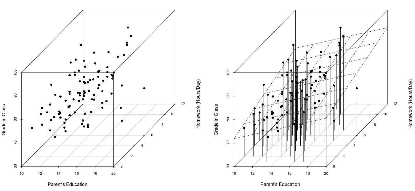
I'll walk you through one using data from a class I'm taking; for now, I'm just going to use R so I can provide good visualization. There are three dimensions here (grades, parents education, and homework); note that this is lame/inappropriate data for this sort of technique, but it'll suffice for illustration.
1. here's the data:
 > str(data2)
 'data.frame':     100 obs. of 3 variables:
  $ grades: num 78 79 79 89 82 77 88 70 86 80 ...
  $ pared : num 13 14 13 13 16 13 13 13 15 14 ...
  $ hwork : num 2 6 1 5 3 4 5 3 5 5 ...

#let's graph it, too
> library(scatterplot3d)
> s3d<-scatterplot3d(new$pared,new$hwork,new$grades, pch=16, xlab="Parent's Education",
  ylab="Homework (Hours/Day)", zlab="Grade in Class", type="h")
>
> model <- lm(grades~pared+hwork) #regress grades on parent education and home work
> s3d$plane(model) #here I just fit the regression plane
The OLS best-fitting plane is shown; it minimizes the squared deviations of actual Grades from Grades predicted from Parent's Education and Homework (Hours/Day).
2. now we've got to subtract the mean from each datum:
 > new<-scale(data2,scale=F)
 >
 > head(new)
    grades pared hwork
 [1,] -2.47 -1.03 -3.09
 [2,] -1.47 -0.03 0.91
 [3,] -1.47 -1.03 -4.09
 [4,]  8.53 -1.03 -0.09
 [5,]  1.53 1.97 -2.09
 [6,] -3.47 -1.03 -1.09
3. ...and calculate the covariance matrix
 > cm<-cov(new)
 > cm
      grades  pared  hwork
 grades 58.110202 4.329192 5.128990
 pared  4.329192 3.726364 1.098283
 hwork  5.128990 1.098283 4.224141
4. ...and calculate the eigenstuff for the covariance matrix
 > eigs<-eigen(cm)
 > eigs
 $values
 [1] 58.946803 4.265718 2.848187
 $vectors
         [,1]       [,2]        [,3]
 [1,] 0.99232104 0.1235818 0.005147218
 [2,] 0.07967798 -0.6068504 -0.790812257
 [3,] 0.09460639 -0.7851498 0.612037156
4.b ...turns out, the
princomp function does this all for you! As a sanity check, lets confirm our eigenguys...
 > pc<-princomp(new, scores=TRUE)
 > pc$loadings

 Loadings:
        Comp.1 Comp.2 Comp.3
 grades 0.992  0.124
 pared        -0.607 -0.791
 hwork        -0.785  0.612
Great, everything looks good!
5. ...check to see which components to keep
 > summary(pc)
 Importance of components:
                        Comp.1    Comp.2    Comp.3
 Standard deviation     7.6391973 2.05500866 1.67919764
 Proportion of Variance 0.8923126 0.06457269 0.04311468
 Cumulative Proportion  0.8923126 0.95688532 1.00000000
A single eigenvector accounts for ~90% of the variance in the data! We'll keep the others around, just to see what happens, but at this point you might eliminate weaker components.
6. ...transform the original data on the basis of the principal components
 > scores <- t(eigs$vectors) %*% t(new)   #multiply transpose of eigenvectors by transpose of original, normalized data
 >
 > head(scores)
       grades    pared    hwork
 [1,] -2.825435 2.7459217 -1.0893718
 [2,] -1.375010 -0.8779460 0.5731118
 [3,] -1.927720 3.6546532 -1.6962618
 [4,] 8.373916 1.7498719 0.8033591
 [5,] 1.477489 0.6345479 -2.8291826
 [6,] -3.628543 1.0520404 0.1295553
Let's visualize our eigenvectors by overlaying them on the transformed data, using the
rgl package
 > library(rgl)
 > plot3d(pc$scores)
 > text3d(6*pc$loadings,texts=colnames(pc$scores),col="red")
 > coords <- NULL
 > for (i in 1:nrow(pc$loadings)) {
 +  coords <- rbind(coords, rbind(c(0,0,0),pc$loadings[i,1:3]))
 + }
 >
 > lines3d(6*coords, col="red", lwd=4)
The interactive plot is much more convincing, so run it yourself! The eigenvectors are the axes of the transformed data, thus providing a better characterization.
In summary, we have transformed our data so that it is expressed in terms of the patterns between them (lines that best describe the relationships among the variables); essentially, we have classified our data points as combinations of the contributions from all three lines, which can be thought of as representing the best possible coordinate system for the data: the greatest variance of some projection of the data comes lies on the first coordinate (called the first principal component), the second greatest variance on the second coordinate, etc.
______________________________________________________
Eigenfaces!
Many face-recognition techniques treat the pixels of a each face-picture as a vector of values; this one does
PCA on many such vectors to abstract characteristic features which can then be used to classify new faces.
Think of an image as a matrix of pixels; let's restrict our attention to grayscale for clarity. Each pixel in a grayscale image is assigned an intensity value from 0 to 255, where "0" is completely black and "255" is completely white. The pictures I am using are 92px by 112px, meaning that there are 92 pixels along each of 112 rows, or equivalently, 112px in each of 92 columns. So, each image comprises a total of 112 * 92 = 10,304 pixels. You can think of each face as a point in a space of 10,304 dimensions! Or rather, you can't very easily think of this, but that's exactly what we've got!
How can we use this information to compute similarities and differences between two pictures? PCA! Take each "row" of pixels in each image and concatenate them to make a single vector of pixel values, like this:
Image vector =<px1 px2 ... px93 px94 ... px10302 px10304>
...where each "px__" is a single pixel with a grayscale intensity value ranging from 0 to 225. At this point, we have a vector full of numbers... a single dimension. Now, the idea is you take a bunch of these image vectors (made from different images), slap them all into a matrix, normalize them, generate a covariance matrix, find the eigenvectors/values for the matrix, and use these values to measure the difference between a new image and the originals. If the distance is small enough (per some threshold value), then a match condition is satisfied!
I'll show you how all of this works in GNU Octave, but the code should work in Matlab too. In Octave, you need to have the images package installed.
First, we need a "training set" of small grayscale images, all the same size. Many computer vision databases exist, with many such sets to choose from. I'm using 200 images from the
AT&T face database (20 subjects, 10 images each).
Here's an example image from the training set, a grayscale image 92 pixels wide by 112 pixels tall (I've got no idea who this guy is):
First, we have to read in
all 200 of these images. I have adapted the procedure from this
Matlab source code, which was really great and required only modest modification: here's
the exact code I ended up using in Octave v3.8
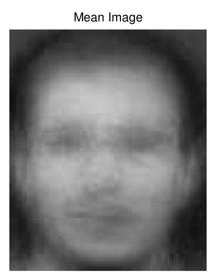
We then take the mean of all of the image vectors, which results in the following image vector:
Good! Now we subtract this mean image from each image in our training-set and compute the covariance matrix exactly as shown in
the discussion above on PCA. The clincher is that for any distribution of data with
n variables, we can describe them with a basis of eigenvectors, and because these are necessarily orthogonal, the variables will be uncorrelated.
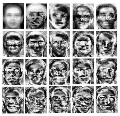
Below are the eigenfaces*, and boy are they ghastly! Think of them as the pixel representation of each eigenvector formed from the covariance matrix of all images; these faces represent the most similar parts of some faces, and the most dramatic differences between others.
*BTW, I think the first one was mistakenly replaced by the mean image in this picture.
Now that we have facespace, how do we go about recognizing a new face? The
recognition procedure is as follows: once we have projected every sample image into
the eigenface subspace, we have a bunch of points in a 20 dimensional space. When given a new image (a new picture of someone in the training set), all we need do is project it into face space and find the smallest distance between the new point and each of the
projections of the sample images: of the people pictured in the training set, this gives us the one that best matches the input picture.
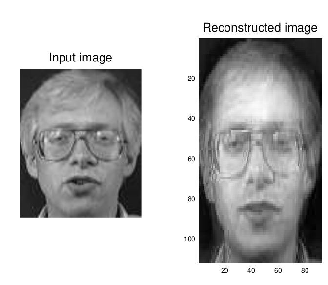
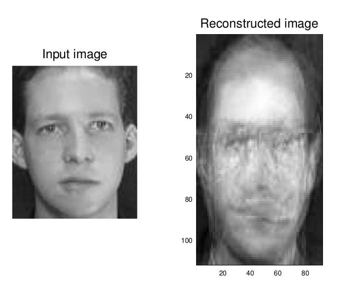
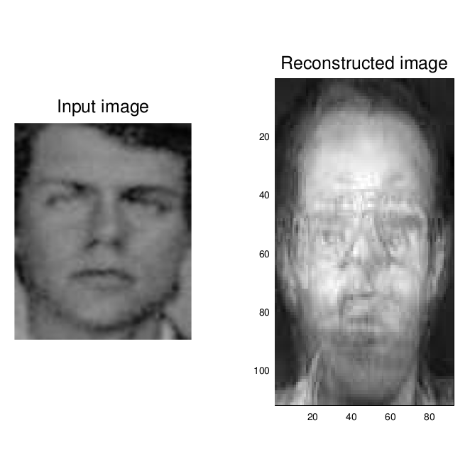
I kept one image of each individual out of the training set for a confirmatory test of our eigenfaces. Here's the first and second input image alongside the image reconstructed from their
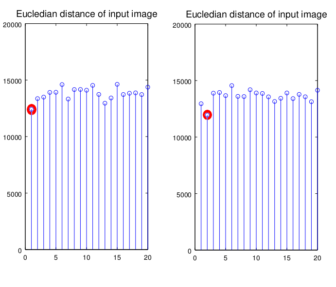
These graphs show the distance of each input image to each person on the training set (along the x-axis, 1-20); both matched! The first input image had the shortest distance to other images of that person, and so did the second (see the red dot in the figure below)!
I decided to try a picture of myself that was already in black and white, to see if it could reconstruct it; with a large enough data set, it could produce a perfect reconstruction, much in the way that Fourier transforms/decompositions work.
Not good at all, really, is it? I probably screwed something up... this is one of my first forays into GNU Octave and I'm just fumbling my way through someone else's Matlab code. Still, we were able to positively classify two untrained images! That's not too bad for a first go.
What could this technique be used for, practically? It's actually
pretty old, and has been largely supplanted by newer, more accurate recognition methods. One immediate use for eigenfaces would be to implement a face-recognition password system for your computer,
like these guys did. You can also use it for face detection, not just recognition.
I'm totally trashed; this took me forever! Like 10 hours! I apologize if I have egregiously misrepresented or oversimplified any of the mathematics involved; I'm way out of my comfort zone with this stuff!
If you're interested in this technique, here's a list of webpages I consulted while writing this post:
http://www.bytefish.de/pdf/facerec_octave.pdf
http://jmcspot.com/Eigenface/Default
https://en.wikipedia.org/wiki/Eigenface
http://www.pages.drexel.edu/~sis26/Eigenface%20Tutorial.htm
http://jeremykun.com/2011/07/27/eigenfaces/
http://codeformatter.blogspot.com/